The Vector Rules in Quantum Mechanics

In today’s post, we introduce the six postulates of quantum mechanics. Together, they establish the vector as the fundamental object of the theory—that which provides the quantum description of a physical system. Quantum mechanics uses lots of jargon, so we will translate specialized terms into those commonly used in linear algebra, the mathematical backbone of the theory that lays down the rules that the system follows. With the six postulates defined, we will then see how quantum mechanics compares to classical theory: we will see that the Hamilton–Jacobi equations and Newton’s second law of motion emerge from quantum mechanics.

Our principal source is the material in chapters 2 and 3 from the textbook Quantum Mechanics by Claude Cohen-Tannoudji, Bernard Diu, and Franck Laloë.

1. Introduction

We begin with the six postulates of quantum mechanics, which define the mathematical framework the theory. To set the mood, here they are in English: 1) The momentary state of a physical system can be described as a vector in an abstract vector space. 2) Each observable quantity of the physical system can be described as a matrix that acts on the state vector through matrix multiplication. 3) When making a measurement, we will apply the matrix for the quantity being measured to the state vector of the system; the matrix has an eigenvalue decomposition, and the outcome of the measurement will always be one of its eigenvalues. 4) The particular outcome observed will be determined randomly: the eigenvalues most likely to be observed are those with eigenvectors best resembling the state vector just before measurement. 5) Right after the measurement, the state vector will abruptly change to match the eigenvector that corresponds to the eigenvalue observed. 6) Between measurements, the state vector smoothly evolves according to a differential equation associated with the total energy of the system.

That’s it. These six sentences form the core of the theory. But the more you think about it—the abrupt, random changes of the system after measurement—the less the world described makes sense. Yet, we cannot discard the theory. As strange as it is, quantum mechanics has passed all experimental tests attempted so far, the most stringent ones requiring precision well beyond any other theory conceived.

In the next section, we will make the postulates more precise by providing some of the mathematics of the theory. The level of rigor will remain informal but should enable us to better appreciate the consequences of the theory. By proceeding in this way, we aim to demonstrate how theoretical physicists go about their work: mathematical theory first, consequences second, and occasionally `What does it all mean?’ third. The rationale for this approach is simple: for all we can see, the rules of nature are written in mathematics, and nature always sticks to her rules. Therefore, good physical theories cannot afford arbitrary qualities; they must be fully constrained by mathematics. The final arbiter about a theory, of course, is experiment. Physical theories ought to make falsifiable predictions, so that they can be rejected if experiment disagrees with their predictions.

2. The Six Postulates

To define the postulates concisely, we consider our system to be a single particle that lives in one space dimension ${x}$ and one time dimension ${t.}$ However, quantum mechanics applies to any system within our universe.

2.1. First: Quantum States

The first postulate tells us that the momentary state of a physical system can be described as a vector in an abstract vector space.

The quantum state of a particle is fully characterized at a given time by a square-integrable wavefunction ${\psi(x).}$ We associate a ket ${\lvert \psi \rangle}$ of the state space ${\cal H}$ with each ${\psi}$ such that

$\displaystyle \psi(x) = \langle x \lvert \psi \rangle. \ \ \ \ \ (1)$

Thus, at fixed time ${t}$ , the state is defined by ${\lvert \psi(t) \rangle \in \cal H.}$

The wavefunction ${\psi(x)}$ is the core idea of quantum mechanics and represents a sharp departure from classical physics. In classical mechanics, we only needed a few real numbers to represent the state of a particle at a given time: its position and velocity coordinates. In quantum mechanics, we need one complex number for every point in space to represent the same particle; that is, we need a whole function ${\psi(x).}$ We made this enormous change because it turns out that particles do not move the way we first thought they did. More information than what is encoded in classical mechanics is needed to fully describe the state of a particle and what it could do next.

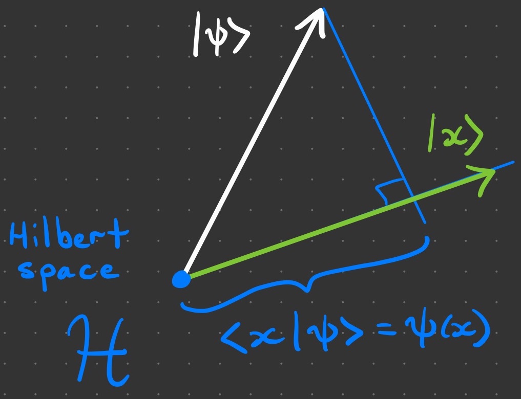
Before getting into this, we need to associate the wavefunction ${\psi(x)}$ with a vector, which we denote by putting funny brackets around the function ${\lvert \psi \rangle.}$ This vector has an infinite number of elements, one for each point ${x}$ in space, and lives in the infinite-dimensional Hilbert space denoted ${\cal H.}$ The funny brackets come from the bra–ket notation, a brilliant invention by Paul Dirac allowing us to easily distinguish column-vectors called kets written as ${\lvert \psi \rangle}$ from row-vectors called bras written as ${\langle \psi \rvert.}$

The bra–ket notation will help us leverage the power of linear algebra operations like the inner and outer products, matrix multiplication, and matrix transposition. For example, the inner product was used in equation (1) to explicitly relate wavefunctions to vectors. We can compute the value of the wave function ${\psi(x)}$ at some point ${x}$ by taking the inner product between ${\lvert \psi \rangle}$ and the position vector ${\lvert x \rangle}$ that essentially has value ${1}$ in the element corresponding to the point ${x}$ and has ${0}$ everywhere else. To take an inner product, we need to transpose one of the vectors before multiplying, and this is what a bra is: ${\langle x \lvert = (\lvert x \rangle)^\dagger}$ , where the dagger represents a fancy transpose called the adjoint. So, ${\langle x \lvert \psi \rangle}$ is indeed the inner product that picks out the the element of ${\lvert \psi \rangle}$ at the point ${x}$ and multiplies it by ${1}$ ; all other elements are multiplied by ${0.}$ The kets ${\lvert \psi \rangle}$ and ${\lvert x \rangle}$ in ${\cal H}$ are sketched below along with an illustration of the computation ${\langle x \lvert \psi \rangle.}$

2.2. Second: Observables

The second postulate tells us that each observable quantity of the physical system can be described as a matrix that acts on the state vector through matrix multiplication.

Every measurable physical quantity ${\cal A}$ is described by an operator ${A}$ acting in ${\cal H.}$ We call ${A}$ an observable. Thus, states are associated with vectors and physical quantities with matrix operators in a vector space.

A measurable quantity can be any number obtained by experiment. We have already seen one such quantity, the position of the particle; call it ${\cal X.}$ The corresponding observable for ${\cal X}$ is the matrix ${X}$ that lives in ${\cal H.}$ So, to measure the position of the particle with wavefunction ${\psi(x)}$ , we would consider the matrix product: ${X \lvert \psi \rangle.}$

Although a matrix multiplying a vector yields another vector, also in ${\cal H}$ , we will soon see that the purpose of the observable is not to transform the vector ${\lvert \psi \rangle}$ but rather to analyze it. For now, we can say that all observables are square matrices whose set of orthogonal eigenvectors span ${\cal H}$ or a proper subset of ${\cal H.}$ Therefore, we can think of the matrix product ${A \lvert \psi \rangle}$ as the observable ${A}$ representing the vector ${\lvert \psi \rangle}$ or its projection in the subspace spanned by the eigenvectors of ${A.}$ This idea will feature prominently in the remaining postulates, so we illustrate this for a generic physical quantity ${\cal A}$ below.

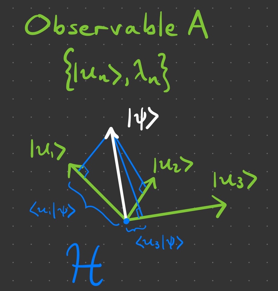
Returning to our familiar example of position ${\cal X}$ , the eigenvectors corresponding of the observable ${X}$ are simply the position vectors ${\lvert x \rangle}$ for each point ${x}$ in space. They are indeed orthogonal from each other. In this case, the set ${\{ \lvert x \rangle \}}$ spans all of ${\cal H}$ , but this need not be the case for a general quantity ${\cal A.}$ As you may have guessed, the quantity ${\cal X}$ is of special importance: it defines space itself! Another important quantity is the momentum of the particle ${\cal P}$ , and we could have written the wavefunction using the set of all possible momentum vectors, such that ${\psi(p) = \langle p \rvert \psi \rangle.}$

The main point is that any physical quantity ${\cal A}$ is associated with a matrix ${A}$ called an observable that provides a basis of eigenvectors for analyzing a state vector ${\lvert \psi \rangle.}$

2.3. Third: Measurement

The third postulate tells that when making a measurement, we must apply the matrix for the quantity being measured to the state vector of the system. The matrix has an eigenvalue decomposition, and the outcome of the measurement will always be one of its eigenvalues.

The only possible outcomes of a measurement of ${\cal A}$ are one of the eigenvalues of ${A.}$ Thus, if ${\lvert u_n \rangle}$ is an eigenvector of ${A}$ with real eigenvalue ${\lambda_n}$ , then measuring ${\cal A}$ entails

$\displaystyle A \lvert u_n \rangle = \lambda_n \lvert u_n \rangle, \ \ \ \ \ (2)$

and the observed outcome is the real number ${\lambda_n.}$

Since the Hilbert space ${\cal H}$ is infinite dimensional, any physical quantity whose eigenvectors span ${\cal H}$ must have an infinite number of eigenvectors. For example, ${X}$ has an infinitude of eigenvectors ${\{ \lvert u_x \rangle = \lvert x \rangle : x \in \mathbf{R} \}.}$ At the other extreme, some physical quantities have very few possible outcomes. For example, the famous Stern–Gerlach experiment measured whether the spin angular momentum of a silver atom was either ${+\frac{\hbar}{2}}$ or ${-\frac{\hbar}{2}.}$ Therefore, the spin quantity ${\cal S}$ has an observable ${S}$ with only two eigenvectors: spin-up ${\lvert u_+ \rangle = \lvert \uparrow \rangle}$ with ${\lambda_+ = +\frac{\hbar}{2}}$ or spin-down ${\lvert u_- \rangle = \lvert \downarrow \rangle}$ with ${\lambda_- = -\frac{\hbar}{2}.}$ In this case, it is implied that the state of the silver atom ${\lvert \psi \rangle}$ also has labels for position and other quantities, but these can be omitted when measuring ${\cal S}$ if the outcome would either fully determine or have no effect on the other quantities.

The definition above labels the set of eigenvectors of ${A}$ as ${\{ \lvert u_n \rangle : n = 1, \ldots, N\}.}$ Were the state of the system ${\lvert \psi \rangle = \lvert u_n \rangle}$ for some ${n \in \{1, \dots, N\}}$ , then the measurement of the quantity ${\cal A}$ would be guaranteed to return the value ${\lambda_n.}$ If we repeated the exact same experiment many times, we would always measure the same value ${\lambda_n.}$ However, were the system a superposition of eigenstates, say ${\lvert \psi \rangle = \frac12 \lvert u_n \rangle + \frac12\lvert u_m \rangle}$ , then it is unclear what the measurement would be. It could either be ${\lambda_n}$ or ${\lambda_m}$ but neither both (surely!) nor anything in between. We will see in the next postulate that the outcome will be purely random.

2.4. Fourth: Random Outcomes

The fourth postulate tells us that the particular outcome observed is determined randomly: the eigenvalues most likely to be observed are those with eigenvectors that best resemble the state vector immediately before measurement.

For simplicity, we assume that ${A}$ has a discrete and non-degenerate eigenvalue spectrum. When a measurement of ${\cal A}$ is made on a system in state ${\lvert \psi \rangle}$ , the probability of observing the outcome ${\lambda_n}$ is given by

$\displaystyle \mathcal{P} (\lambda_n) = \lvert \langle u_n \lvert \psi \rangle \rvert^2, \ \ \ \ \ (3)$

where vectors are normalized to unit length ${\langle \psi \lvert \psi \rangle = \langle u_n \lvert u_n \rangle = 1.}$

That we cannot predict the outcome of a single measurement with certainty—even with perfect information about the system—is a radical departure from classical, deterministic physics. However, the randomness of individual outcomes does not imply that there is no order in the universe and that nothing is predictable. This postulate tells us that we can predict quantitatively how the measurements from a large number of repeated experiments will be distributed across the range, or spectrum, of possible outcomes.

The above paragraph interprets the left-hand side of equation (3), namely, the probabilities ${0 \leq \mathcal{P} (\lambda_n) \leq 1.}$ Let us now think about how the right-hand side of the equation calculates these probabilities. First, we see an inner product between the ${n^\mathrm{th}}$ eigenvector ${\vert u_n \rangle}$ and the state vector ${\lvert \psi \rangle.}$ In words, the inner product ${\langle u_n \lvert \psi \rangle}$ tells us what these two vectors have in common, or somewhat more precisely, the amplitude of the projection of one vector onto the other. Because the Hilbert space ${\cal H}$ represents complex-valued wavefunctions ${\psi(x)}$ and is a complex vector space, its inner product is in general also complex-valued. This is why we see the absolute value bars around the inner product in equation (3), so to yield a non-negative real number. Probabilities only make sense for numbers in the unit interval ${[ 0, 1] }$ , which explains why all state vectors and eigenvectors must always have unit length. Finally, there is a square in the expression ${\lvert \langle u_n \lvert \psi \rangle \rvert^2.}$ Without the square, we still would have probabilities in the unit interval—but they would disagree with experiment. What we do know is the probability of observing a particular outcome goes as the square of the amplitude. That the exponent is exactly ${2}$ suggests a geometrical justification, like an inverse-square law, where probability is conserved in toto but spreads out over some surface area.

There is also an important case when the state of the system is exactly equal to one of the matrix eigenvectors ${\lvert \psi \rangle = \vert u_i \rangle.}$ Then, the prediction is that the probability of observing ${\lambda_n}$ is ${1}$ , and the probability of observing any other eigenvalue is ${0.}$ This turns out to be a crucial point for quantum mechanics, as we will see in the next postulate, which leads to the following sensible behavior. Were we to make a rapid succession of measurements, the first outcome observed would be random for general ${\lvert \psi \rangle}$ , but subsequent outcomes would be identical to the first. Thus, measurement affects the system by immediately putting it in a state consistent with the outcome. This process involving measurement, probability, and collapse is illustrated below.

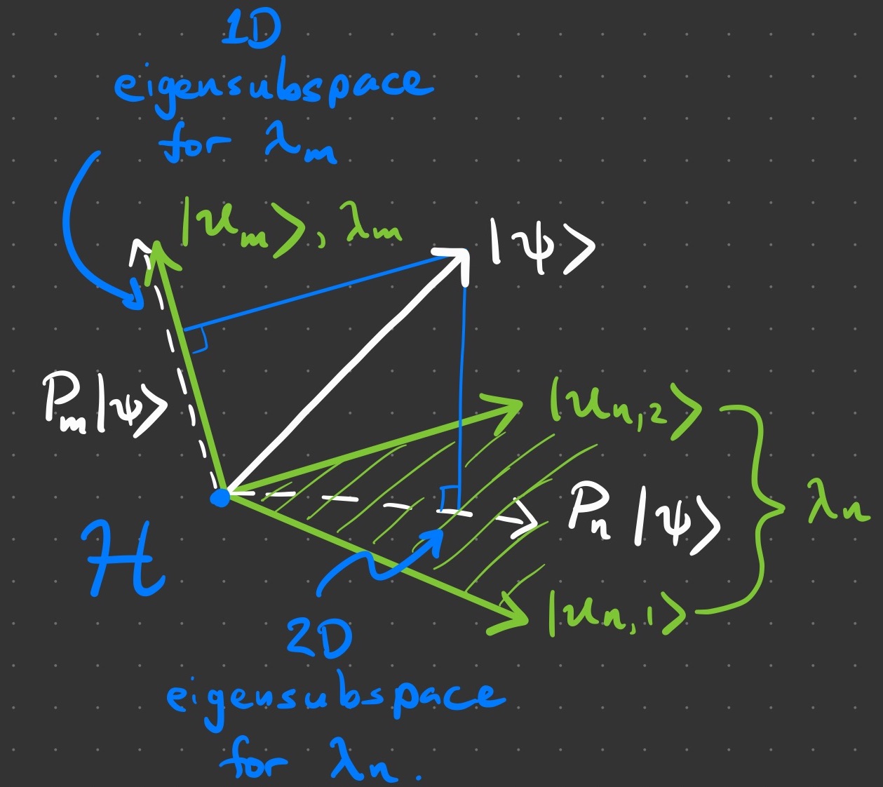
2.5. Fifth: Wavefunction Collapse

The fifth postulate tells us that right after the measurement, the state vector abruptly changes by becoming equal to the matrix eigenvector corresponding to the eigenvalue that was observed.

If the measurement of ${\cal A}$ on the system in state ${\lvert \psi \rangle}$ yields the result ${\lambda_n}$ , then the state immediately after the measurement becomes the normalized projection of ${\lvert \psi \rangle}$ onto the eigensubspace associate with ${\lambda_n}$

$\displaystyle \lvert \psi \rangle \xrightarrow{\lambda_n} \frac{P_n \lvert \psi \rangle}{\sqrt{\langle \psi \lvert P_n \rvert \psi \rangle}}. \ \ \ \ \ (4)$

In the non-degenerate case, the eigensubspace is ${1\mathrm D}$ , thus, ${\lvert \psi \rangle \xrightarrow{\lambda_n} \lvert u_n \rangle.}$

Here we see explicitly how measurement changes the wavefunction ${\lvert \psi \rangle.}$ While in general, the system state may be in some superposition of possible measurement outcomes, the act of measurement immediately puts the system into a state compatible with the observed outcome ${\lambda_n}$ and incompatible with all other alternative outcomes ${\lambda_m}$ for ${m \neq n}$ , as prescribed in the mapping (4). This measurement-induced state change is known as wavefunction collapse because it destroys any superposition of outcome states the system may have occupied before measurement.

The mapping shown in (4) uses the projection operator ${P_n}$ corresponding to the observed eigenvalue ${\lambda_n.}$ In the simplest case, there is only one eigenvector ${\lvert u_n \rangle}$ where ${A \lvert u_n \rangle = \lambda_n \lvert u_n \rangle.}$ This is called the non-degenerate case, and the mapping must simply be ${\lvert \psi \rangle \rightarrow \lvert u_n \rangle.}$ Notice how this would happen if the operator is ${P_n = \lvert u_n \rangle \langle u_n \rvert.}$ Here, we really appreciate the power of the bra–ket notation. A ket (column vector) multiplying a bra (row vector) gives a matrix (an outer product), which is indeed an operator! The numerator of the mapping (4) becomes ${P_n \lvert \psi \rangle = \lvert u_n \rangle \langle u_n \rvert \psi \rangle.}$ This is nothing more than the ket ${\lvert u_n \rangle}$ scaled by the inner product ${\langle u_n \rvert \psi \rangle}$ , i.e., a number. Notice also that the inner product cannot be zero for this mapping because the fourth postulate states that the probability in equation (3) of observing ${\lambda_n}$ would also be zero. Finally, plugging the outer product in for ${P_n}$ in the denominator of (4) yields ${\sqrt{\langle \psi \lvert P_n \rvert \psi \rangle} = \sqrt{(\langle u_n \lvert \psi \rangle)^\star \langle u_n \rvert \psi \rangle} = \sqrt{| \langle u_n \rvert \psi \rangle |^2} = \langle u_n \rvert \psi \rangle}$ , where the star denotes the complex conjugate and reverses the order of the bra and ket. Well, this cancels the inner product in the numerator, giving us exactly what we came for, ${\lvert u_n \rangle.}$

We bothered ourselves with the projection operator because, in general, an eigenvalue ${\lambda_n}$ will correspond to subspace spanned by two or more eigenvectors, such that ${A \lvert u_{n,k} \rangle = \lambda_n \lvert u_n \rangle}$ holds for ${k = 1, 2, \ldots}$ In this case, the operator ${P_n}$ must do something fancier than ${\lvert \psi \rangle \rightarrow \lvert u_n \rangle.}$ It must project ${\lvert \psi \rangle}$ onto the eigensubspace spanned by ${\{ \lvert u_{n,k} \rangle: k = 1, 2, \ldots \}}$ by keeping the components of ${\lvert \psi \rangle}$ that are compatible with ${\lambda_n}$ and setting the rest to zero. This is achieved if we generalize our projection operator to be the sum ${P_n = \sum_k \lvert u_{n,k} \rangle \langle u_{n,k} \rvert.}$ Notice how this collapses back to the simple case for ${k = 1.}$ The action of a projector onto a ${2\mathrm D}$ subspace is illustrated below. You can check that the mapping (4) has unit length in this case, too.

2.6. Sixth: Wavefunction Evolution

The sixth postulate tells us that between measurements, the state vector smoothly evolves according to a differential equation associated with the system’s total energy.

The evolution of the state ${\lvert \psi(t) \rangle}$ is governed by the Schrödinger equation

$\displaystyle \mathrm{i} \hbar \frac{\mathrm{d}}{\mathrm{d} t} \lvert \psi(t) \rangle = H(t) \lvert \psi(t) \rangle, \ \ \ \ \ (5)$

where ${H(t)}$ is the Hamiltonian operator, the observable associated with the total energy of the system. An important example is the spinless particle of mass ${m}$ in a scalar potential ${V(x)}$ , which has the Hamiltonian

$\displaystyle H = \frac{p^2}{2 m} + V(x). \ \ \ \ \ (6)$

The sixth and final postulate establishes the dynamics of quantum mechanics. The Schrödinger equation (5) is a linear first-order differential equation in time that prescribes the state vector ${\lvert \psi \rangle}$ at some moment, say ${t_0}$ , to be the value of the function ${\lvert \psi(t_0) \rangle = \lvert \psi \rangle}$ at ${t=t_0.}$ The function ${\lvert \psi(t) \rangle}$ must satisfy the differential equation (5), whose solutions are determined by the Hamiltonian operator ${H(t)}$ , also a function of time in general. A lot of physics is encoded into equations (5) and (6). Perhaps most important is the appearance of the Planck constant ${\hbar}$ , whence the term quantum (see the post Everything Waves). Here, we touch on the relevant points to our discussion.

First, ${H(t)}$ is indeed an observable acting on ${\lvert \psi(t) \rangle.}$ Like all observables, ${H(t)}$ has an eigenvalue decomposition. Its eigenvalues quantify the all-important total energy of the system, thus their special symbol ${E_n(t)}$ instead of our generic ${\lambda_n.}$ When the total energy is constant, then the system is said to be conservative, and we simply write the Hamiltonian as ${H}$ with eigenvalue spectrum ${\{\lvert \phi_n \rangle, E_n : n = 1,2,\ldots\}.}$ The energy of a conservative system transforms without loss from kinetic to potential and back again, such as in the case of a particle trapped in a potential well ${V(x)}$ with kinetic energy ${p^2 / 2m.}$ This is what is prescribed by equation (6).

Second, as mentioned before, the position ${x}$ and momentum ${p}$ are actually observables. It is sensible to rewrite equation (6) in terms of the matrix operators ${X}$ and ${P}$ ; notice how ${P^2 = P P}$ immediately makes sense as a matrix acting on the state vector ${\lvert \psi(t) \rangle.}$ It will also be of central importance to make the connection between the variables ${x,\,p}$ and the observables ${X,\,P}$ when we explore the quantum origin of classical mechanics in the next section.

Finally, it is worth considering solutions to the Schrödinger equation for constant Hamiltonian ${H.}$ Suppose at time ${t_0}$ we had ${\lvert \psi(t_0) \rangle = \lvert \phi_n \rangle.}$ Then a measurement of the total energy would yield ${H \lvert \phi_n \rangle = E_n \lvert \phi_n \rangle}$ , and ${\lvert \psi(t_0) \rangle}$ would consequently not change. The general solution to the Schrödinger equation (being of first-order) has an exponential form ${\lvert \psi(t) \rangle = e^{-\mathrm{i} E_n (t - t_0)} \lvert \psi(t_0) \rangle}$ , varying only by a global phase factor. Although the global phase rotates over time, it has no effect on any observable because the square of the amplitude will always replace it by ${1.}$ Therefore, states ${\lvert \psi(t) \rangle}$ at different times are always physically indistinguishable. Had we started with the more general case, a superposition of eigenstates ${\lvert \psi(t_0) \rangle = \sum_n c_n \lvert \phi_n \rangle}$ , then our solution to the Schrödinger equation (being linear) would involve relative phase factors ${\lvert \psi(t) \rangle = \sum_n e^{-\mathrm{i} E_n (t - t_0)} \lvert \psi(t_0) \rangle.}$ Relative phases will interfere before the amplitude is squared, so states ${\lvert \psi(t) \rangle}$ at different times are in fact physically distinguishable.

So much for the postulates of quantum mechanics. It would be natural to feel uneasy with the caricatural presentation given here. Indeed, this is no substitute for a rigorous course of study. Having seen the core of the theory will hopefully help you decide whether to follow the rabbit hole any deeper.

3. Classical Mechanics Redux

In this final section, we derive the laws of classical mechanics using what we have learned above. We will also need new material, but don’t sweat it if you have not seen it before; consider it an opportunity to dig deeper. Our goal here is merely to illustrate how the classical emerges from the quantum without diving into detail.

We begin with our observables for position ${X}$ and momentum ${P}$ and compute their expectation, or mean values,

$\displaystyle \langle X \rangle (t) = \langle \psi(t) \lvert X \rvert \psi(t) \rangle, \ \ \ \ \ (7)$

$\displaystyle \langle P \rangle (t) = \langle \psi(t) \lvert P \rvert \psi(t) \rangle. \ \ \ \ \ (8)$

Notice how the bra–ket notation makes it clear that each expectation is simply a scalar function of time, very much how we describe a classical particle using ${x(t)}$ and ${p(t).}$ These expectations are the average position and momentum obtained by repeating many experiments measuring ${\cal X}$ and ${\cal P}$ of our system in state ${\lvert \psi(t) \rangle.}$

We would like to know the dynamics for these operators of average position and momentum. The dynamics are the rules that determine how our system goes from one state to the next; they are known as the equations of motion.

Given a system with Hamiltonian ${H}$ , the equations of motion for any constant operator ${A}$ were found by Werner Heisenberg to be

$\displaystyle \mathrm{i} \frac{\mathrm{d}}{\mathrm{d} t} A = [ A, H ], \ \ \ \ \ (9)$

where ${[A, H] = A H - H A}$ is called the commutator of ${A}$ and ${H.}$

Let us take a moment to discuss commutation relations between operators because they are extremely important in quantum mechanics. Operators are represented as matrices, so the order of matrix multiplication matters, unlike scalars which always commute (e.g., ${xy = yx}$ ). A non-vanishing commutation relation implies that the eigenstates of the two operators are not compatible, so the system cannot simultaneously be in an eigenstate for both operators. Therefore, a non-vanishing commutation relation between two operators means that you cannot measure both quantities simultaneously. The most famous example comes from the Heisenberg uncertainty principle, which states that one cannot measure position and momentum simultaneously. This is encoded in the all-important canonical commutation relations

$\displaystyle [X_i, P_j] = \mathrm{i} \delta_{ij}, \ \ \ \ \ (10)$

where ${i,j}$ index the spatial directions ${x,y,z}$ , and ${\delta_{ij} = 1}$ for ${i=j}$ and ${0}$ otherwise is called the Kronecker ${\delta}$ -function.

Now, let us return to the task at hand. Our system has Hamiltonian operator

$\displaystyle H = \frac{P^2}{2 m} + V(X), \ \ \ \ \ (11)$

and we can plug our ${\langle X \rangle}$ and ${\langle P \rangle}$ operators in place of ${A.}$ Notice that any operator ${A}$ commutes with itself, i.e., ${[A, A] = 0.}$ This implies that ${[X, V(X)] = 0}$ as well as ${[P, P^2] = 0.}$ Altogether, we find our equations of motion become

$\displaystyle \mathrm{i} \frac{\mathrm{d}}{\mathrm{d} t} \langle X \rangle = \big\langle [ X, H ] \big\rangle = \Big\langle \Big[ X, \frac{P^2}{2m} \Big] \Big\rangle, \ \ \ \ \ (12)$

$\displaystyle \mathrm{i} \frac{\mathrm{d}}{\mathrm{d} t} \langle P \rangle = \big\langle [ P, H ] \big\rangle = \big\langle [ P, V(X) ] \big\rangle. \ \ \ \ \ (13)$

Using the canonical commutation relations in equation (10), the commutator in the equations of motion for position (12) is

$\displaystyle \Big\langle \Big[ X, \frac{P^2}{2m} \Big] \Big\rangle = \frac{1}{2m} \big( [X,P] P + P [X, P] \big) = \frac{\mathrm{i}}{m} P. \ \ \ \ \ (14)$

The commutator in the equations of motion for momentum (13) is found using the correspondence between the momentum and differential operators ${P \leftrightarrow -\mathrm{i} \nabla}$ , yielding

$\displaystyle \langle [ P, V(X) ] \rangle = - \mathrm{i} \big(\nabla V(X) - V(X) \nabla \big) = -\mathrm{i} \nabla V(X). \ \ \ \ \ (15)$

Restoring these results into the equations of motion (12) and (13) reads

$\displaystyle \frac{\mathrm{d}}{\mathrm{d} t} \langle X \rangle = \frac{1}{m} \langle P \rangle, \ \ \ \ \ (16)$

$\displaystyle \frac{\mathrm{d}}{\mathrm{d} t} \langle P \rangle = -\big\langle \nabla V(X) \big\rangle, \ \ \ \ \ (17)$

which is known as Ehrenfest’s theorem in quantum mechanics.

By interpreting the averages of the position and momentum operators as the scalar variables of classical mechanics, ${\langle X \rangle \leftrightarrow x}$ and ${\langle P \rangle \leftrightarrow p}$ , we find the Hamilton–Jacobi equations of classical mechanics, as advertised. Combining these two equations, we obtain Newton’s second law of motion, where force is defined as the rate-of-change of momentum or, equivalently, as the negative of the gradient of the potential

$\displaystyle \frac{\mathrm{d} p}{\mathrm{d} t} = m \frac{\mathrm{d}^2 x}{\mathrm{d} t^2} = - \nabla V(x) \quad \Longleftrightarrow \quad F = ma. \ \ \ \ \ (18)$

Share this:

Related

Leave a comment