How Theory Predicts Antimatter

This first post is representative of the articles that will follow. Informally written for undergraduate students, it aims to offer the reader a sense of what modern particle physics is like. We will discuss the theoretical prediction of the positron to illustrate how results in our subject sometimes come about. Typically, we begin with a few physical assumptions and try to find a sequence of mathematical arguments that leads us to inevitable conclusions. Special relativity and quantum mechanics also appear here with a character similar to that when invoked in formal arguments.

This particular example is adapted from the material in chapters 8 and 9 from the textbook Quantum Field Theory and the Standard Model by Matthew D. Schwartz.

1. Introduction

In this post, we will be exploring the theory of electrons and light. By considering how electrons interact with light, we will arrive at the inevitable conclusion that this can happen only if the electron co-exists with another particle in the universe that is uniquely associated with it. This new particle is called the positron and is in fact the anti-particle of the electron.

2. About the electron

We will proceed with an approximation of the electron. The electron is a point-like particle with a fixed mass ${m}$ and charge ${-e}$ . In reality, the electron has one more property called spin, but we will ignore this here as it unnecessarily complicates our discussion without affecting the result.

Because there is nothing else to the electron, we can represent it and its behavior by a quantum scalar field that takes on one value at each point in spacetime, which we write as the four-dimensional vector ${x^\mu = (t, \vec x)}$ . A particle exists wherever this field is excited. We write this scalar-valued field as

$\displaystyle \phi = \phi(x^\mu). \ \ \ \ \ (1)$

3. About light

We have discovered that light has a property called polarization. Light is an electromagnetic wave, such that its electric and magnetic components undulate at right angles of each other. So, there are two axes that must be chosen in the three dimensions of space in order to unambiguously determine the polarization of the light. We therefore say that light has two degrees of freedom.

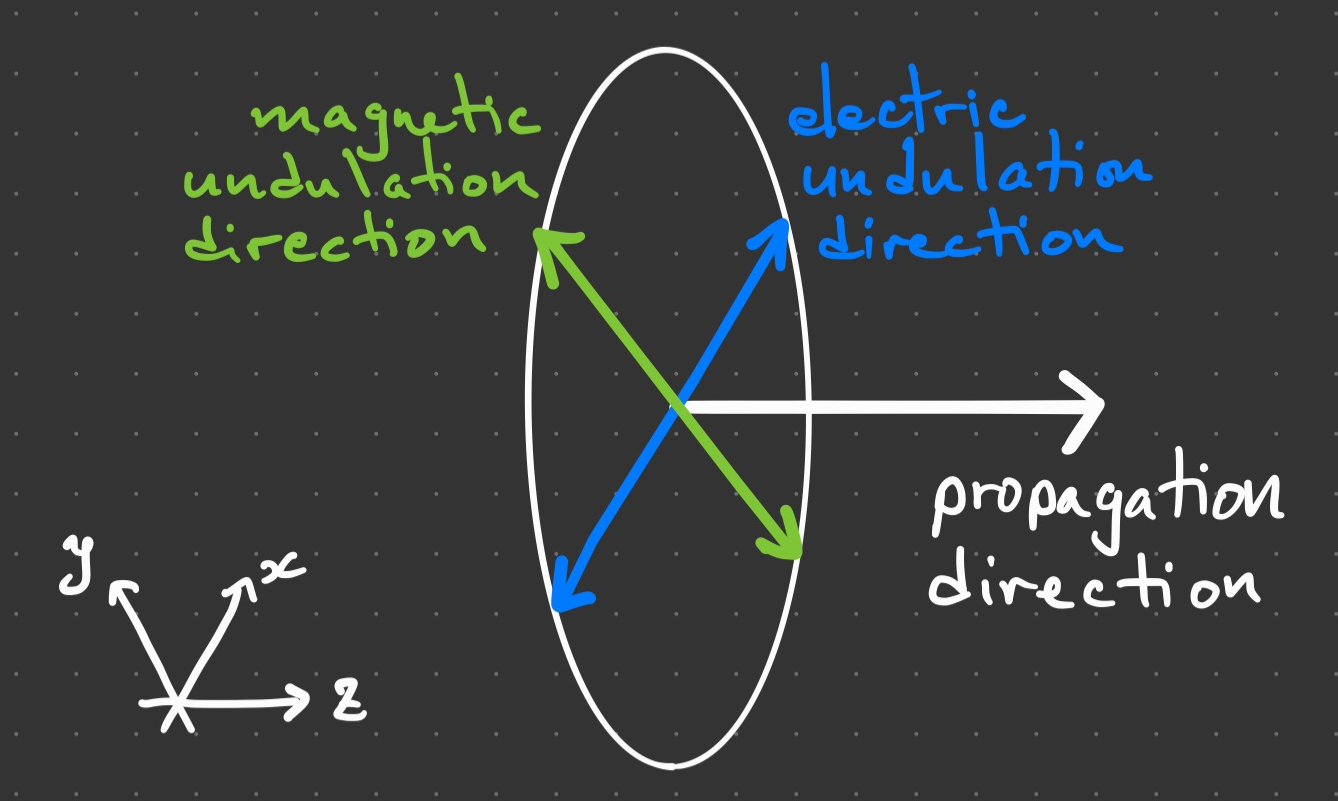
This polarization carries over to the quantum field that gives rise to the individual particles of light called photons. Therefore, the quantum field for the photon must be a vector quantity so to be able to encode the two degrees of freedom at each point of spacetime. We write this quantum vector field as

$\displaystyle A^\mu = A^\mu(x^\mu). \ \ \ \ \ (2)$

It is important to note that the vector ${A^\mu}$ stores a value for the time coordinate ${t}$ and each of the three spatial coordinates ${\vec x = (x, y, z)}$ . Since there can only be two degrees of freedom for the photon, this means that the four values in ${A^\mu}$ must be correlated in a special way. This special relationship amounts to the property called gauge invariance, which means that there are certain mathematical transformations of ${A^\mu}$ that have no physical effect on the photon. We will explore the properties of these transformations in the next section. For now, think of these transformations as the addition of another vector field ${\partial^\mu \alpha}$ . Gauge invariance means that the transformation

$\displaystyle A^\mu \longrightarrow A^\mu + \partial^\mu \alpha \ \ \ \ \ (3)$

has no effect on the outcome of any physical calculation.

4. Physical description of the system

A complete physical description of a system is given by a function of its energy called the Lagrangian density. For our particular system, the electron and photon quantum fields become the independent variables of the Lagrangian. It is written as

$\displaystyle \mathcal{L} (\phi, A^\mu) = \cdots \ \ \ \ \ (4)$

and includes a series of terms depending on ${\phi}$ and ${A^\mu}$ quantifying the kinetic and potential energy of the system as well as terms describing how the particle fields interact.

A key property of the Lagrangian is its independence from the observer, which means that it is unaffected by Lorentz transformations that take us from one spacetime coordinate reference frame to another. This is known as Lorentz invariance. Furthermore, the Lagrangian for any photon theory must also be gauge invariant. This follows from the premise that a gauge transformation takes us to distinct but physically redundant formulation of the electromagnetic field.

The invariance properties just discussed constrain how the four elements of the vector ${A^\mu}$ are allowed to mix among each other. An intuitive way to think about how these transformations are related is to accept that Lorentz transformations generally mix up three polarization axes, but light only has two polarization axes. Thus, gauge transformations introduce redundancy by preventing the two axes of light from getting mixed up with a third, unphysical, axis.

That the Lagrangian respects both Lorentz invariance and gauge invariance is a direct consequence of the assumptions of the special theory of relativity:

Physics is the same for different inertial observers.
Light always travels at the maximum speed limit in the vacuum relative to all possible observers.

5. Interaction of the electron and the photon

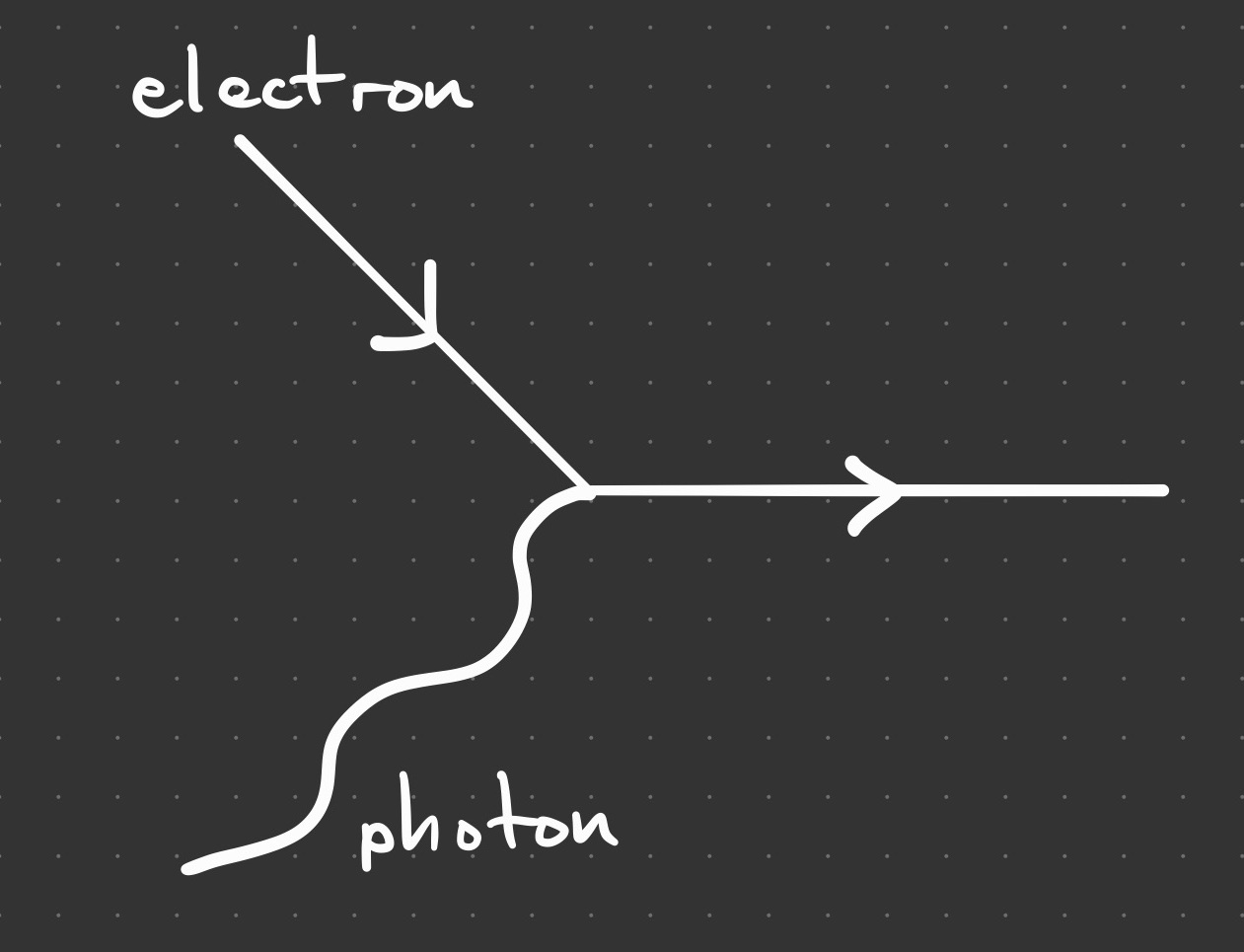
Now we will see why coupling the electron and the photon leads to trouble. An interaction occurs at a point in spacetime where two particles make contact. A photon can interact with an electron as shown in the diagram.

This is a problem because any interaction term will involve factors like ${A^\mu \phi}$ that violates the invariance property of the Lagrangian, as we will see next. If we perform a gauge transformation on the photon ${A^\mu \rightarrow A^\mu + \partial^\mu \alpha}$ , the interaction becomes

$\displaystyle A^\mu \phi \longrightarrow (A^\mu + \partial^\mu \alpha) \phi = A^\mu \phi + (\partial^\mu \alpha) \phi. \ \ \ \ \ (5)$

But now the Lagrangian has changed by taking a new term ${(\partial^\mu \alpha) \phi \neq 0}$ that is non-zero in general.

Intuitively, we can understand why this happens. A gauge transformation mixes up the elements of ${A^\mu}$ . But if ${\phi}$ is just a real (scalar) number, then there is no way for it to counterbalance or compensate the changes in ${A^\mu}$ in order to leave the Lagrangian invariant. Therefore, the electron quantum field ${\phi}$ cannot simply be a real scalar. We need more freedom.

6. Adding another degree of freedom to the electron field

It turns out that including one additional real scalar to the electron field is enough to restore invariance in the Lagrangian. The electron quantum field can therefore be re-written as a complex (though still a scalar) number

$\displaystyle \phi(x^\mu) = \phi_1(x^\mu) + \mathrm{i} \phi_2(x^\mu) \ \ \ \ \ (6)$

or equivalently (and more conveniently) as the distinct conjugate pair ${\phi(x^\mu)}$ and ${\phi^\star(x^\mu)}$ , where we require

$\displaystyle \phi(x^\mu) \neq \phi^\star(x^\mu). \ \ \ \ \ (7)$

To understand the consequences of this requirement, we must take a closer look at what a quantum field is. The quantum field for a particle is mathematically formulated as a combination of operators ${a_p^\dagger}$ and ${a_p}$ , respectively associated with the creation and the annihilation of the particle

$\displaystyle \phi(x^\mu) = \int \frac{\mathrm{d}^3 p}{(2\pi)^3} \frac{1}{\sqrt{2\omega_p}} (a_p e^{-\mathrm{i} p x} + a_p^\dagger e^{\mathrm{i} p x}). \ \ \ \ \ (8)$

There is a lot of information encoded in this equation, but you need not understand it all now. Just consider that the field value at the point ${x^\mu}$ is obtained by considering both the creation and annihilation of a particle of arbitrary momentum.

Because a particle can be created or annihilated with any quantity of energy-momentum, quantified by the four-element vector ${p}$ , the field operator is defined as an integral. It is important to note that the creation and annihilation operators for a particle are conjugates of each other:

$\displaystyle (a_p)^\dagger = a_p^\dagger \quad\textrm{and}\quad (a_p^\dagger)^\dagger = a_p. \ \ \ \ \ (9)$

Now, if we attempt to take the conjugate of the electron quantum field, the creation and annihilation operators and their complex exponentials ${e^{ipx}}$ merely trade places, and nothing changes: ${\phi^\star(x^\mu) = \phi(x^\mu)}$ . So this will not do. This equality can be broken by introducing a new operator ${b_p}$ , such that the creation and annihilation operators are no longer conjugates of each other

$\displaystyle (a_p)^\dagger \neq b_p^\dagger. \ \ \ \ \ (10)$

Something remarkable has just happened! The conjugate scalar fields are now distinct, with the creation of one particle coupled to the annihilation of a new particle represented by the operator ${b_p}$ :

$\displaystyle \phi(x^\mu) = \int \frac{\mathrm{d}^3 p}{(2\pi)^3} \frac{1}{\sqrt{2\omega_p}} (a_p e^{-\mathrm{i} p x} + b_p^\dagger e^{\mathrm{i} p x}) \ \ \ \ \ (11)$

$\displaystyle \phi^\star(x^\mu) = \int \frac{\mathrm{d}^3 p}{(2\pi)^3} \frac{1}{\sqrt{2\omega_p}} (a_p^\dagger e^{\mathrm{i} p x} + b_p e^{-\mathrm{i} p x}) \ \ \ \ \ (12)$

This new particle, however, is anything but a freebie. Its properties are already fully constrained by the modified—and now invariant—Lagrangian ${\mathcal{L}(\phi, \phi^\star, A^\mu)}$ . Too involved to show here, the following properties emerge. The Lagrangian prescribes exactly the same dynamics for both particles. Both particles have exactly the same mass ${m}$ . The only difference is the new particle’s opposite electrical charge ${+e}$ .

In addition to all of this, because the creation and annihilation of this new particle are inextricably tied to those for the electron, we refer to it as the electron’s anti-particle, also known as the positron. Indeed, positrons were eventually discovered to have exactly the same properties predicted above.

7. Special Relativity ${+}$ Quantum Mechanics ${\rightarrow}$ Antimatter

To summarize, the assumptions of special relativity have the consequences of Lorentz invariance and gauge symmetry. And the assumptions of quantum mechanics have the consequences of the creation and annihilation of discrete particles. Taken together, these assumptions imply that all matter that interacts with light must also exist in the form of antimatter.

This post attempts to expose you to some of the ways of thinking in theoretical physics. We hope that you can appreciate how even a small number of assumptions, when carefully applied to mathematical reasoning, can lead to inevitable and remarkable facts about the world.

Share this:

Related

Leave a comment